Hardware-in-the-loop simulation of the booster catch maneuver
Not affiliated
Last updated
Overview
This project explores the development of autonomous control software for the Super Heavy booster to perform a precise catch maneuver, by reverse-engineering the real system (looking at how it works, at public materials, and proving this solution is plausible). The simulation environment models the booster dynamics, atmospheric effects, and the mechanical behavior of the catch mechanism. Going beyond a simple simulation, the maneuver will happen live in a FANUC robotic cell with human-sized mockups, equipped with noisy sensors and actuators: a hardware-in-the-loop simulation. This makes the simulation susceptible to real noise, drift, and imprecision. It also helps me interest people in the project: it is much more entertaining to see a rocket fly than a cylinder move on a screen.
This is a robotics engineering study project at Polytech Dijon. Robotics is everything that has sensors, actuators, and compute, so even rockets fall into our field. This study project is a perfect fit for me: it brings together passion, advanced theoretical fields, and real-world applications. Crazy as it is, my tutor accepted my project in only a few minutes.
Space exploration is awe-inspiring, and is becoming the obvious next civilization step. The innovations a system like Starship is bringing are crucial for a meaningful adventure into space, for humans and for the economy. Man used to work on cathedrals they would never see completed, and I qualify space exploration as today's cathedral, and I want to be part of it.
Starting at 40 km altitude (~130k ft) on a ballistic trajectory a small distance short of the launch site, the booster will go through 3 phases:
Descent at high speeds (up to Mach 4)
Decelerate using 13 engines
Set itself down on two arms mounted on the launch tower with 5 engines
This requires multiple guidance methods (aerodynamic surfaces and thrust vector control), and a solid control system.
Simulation & Control Software : ProxSim
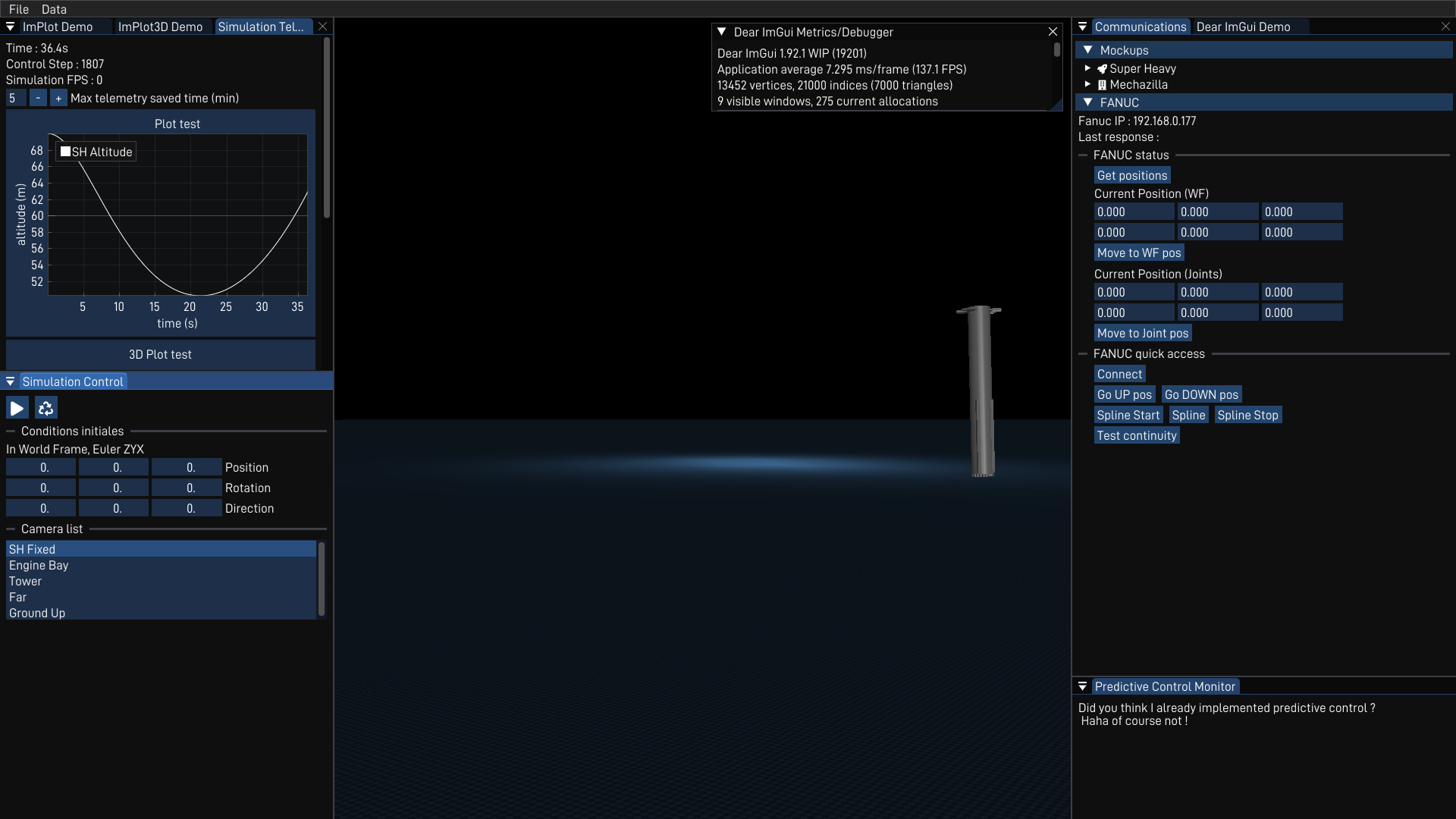
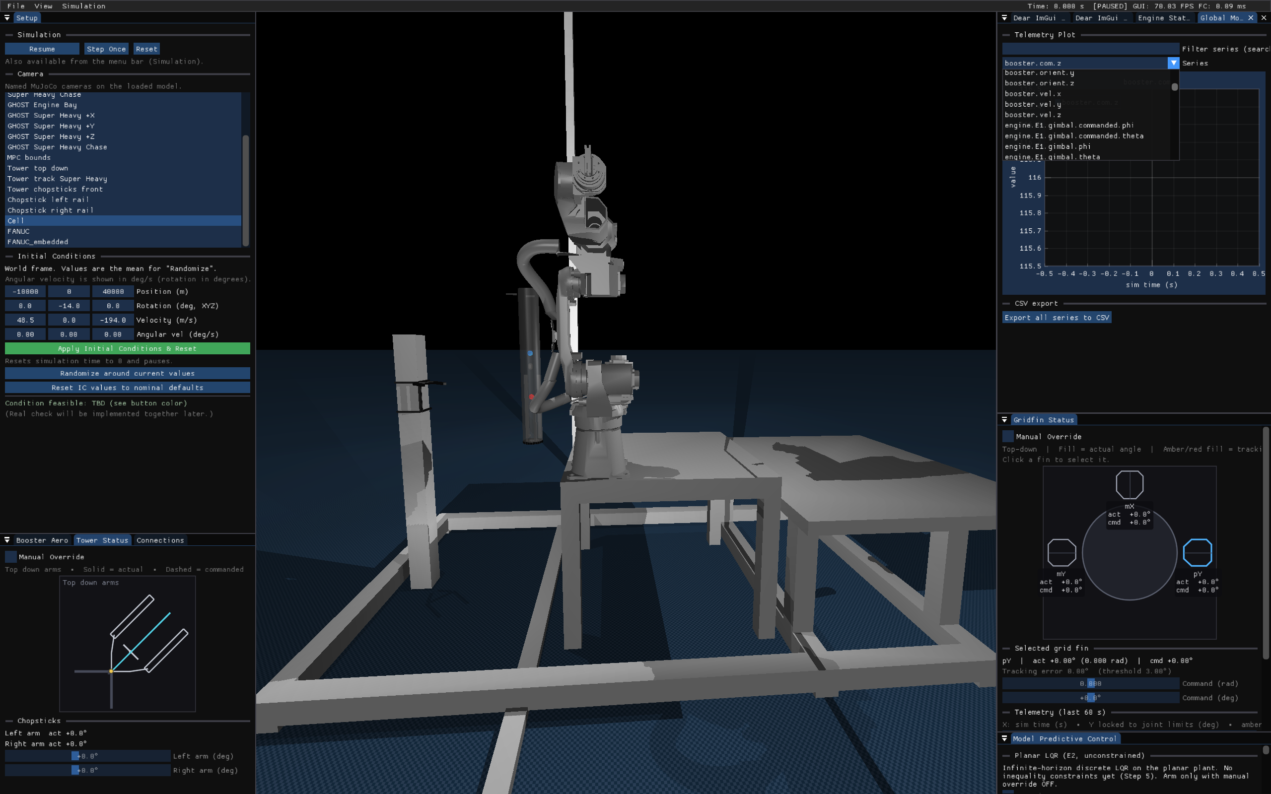
I need an environment where the physics simulation happens, and where it can send movements and receive sensor data. This is why I made my own software in C++, using MuJoCo for the physical simulation, and ImGui for the interface. MuJoCo is an open-source simulation engine that is widely used in AI robotics at Nvidia and Google DeepMind, and ImGui is a widely used open-source library for building user interfaces in C++. Applying multiple meganewtons of force on rotating engines and keeping the simulation stable was a difficult job.
Screenshot of ProxSim while a simulation was running with a Super Heavy V3. Camera control, telemetry, vehicule commands, and ghost booster display.
The whole goal of "control" is to tell the booster what to do by itself. This problem is unpredictable and it needs to work even if an engine can't start, if there is cross-wind, or if a grid fin is stuck; it is a sort of sentience. As of today, a simple controller (PID) is implemented to hold the booster upright, far from the end goal: Model Predictive Control.
Model Predictive Control (MPC) is a state representation of a system, and an optimization algorithm. Given a state X of the system and its model (A, B, C, D) (a physical model such as mass, inertia, and response to commands), it estimates the future in order to reach a setpoint.
{X˙=AX+BUY=CX+DU
A is the free response of the system (given no command, the booster simply falls). B is how the system behaves in response to commands (torque, force, fuel consumption). C is what is measurable (the position of the booster is measurable, and is a goal/setpoint of the controller). D is often 0 (the command has no direct consequences).
Details about MPC
MPC with constraints (thrust bounds, gimbal directions, not hit the tower...), can't be solved analytically, it is an optimization problem instead. Given a cost function J, we need to find the least costly (the cost can be precision, fuel consumption ...) solution to "converge" to.
One of the greatest issues in optimization is dealing with "non-convex" problems, as it implies that the found solution we converge to might not be the optimal solution : stuck in a local minima while searching for the global minima.
This Soft Landing problem has non-convexities coming from thrust vectors when gimballing and a variable thrust is possible for example, and this is solved by Lossless Convexification, a paper from Lars Blackmore, who worked on SpaceX's Falcon 9 landing control and today's Starship upper stage control.
Lossless Convexification proposes a re-formulation of the Soft Landing problem that is convex, and enables optimization algorithms to find the optimal solution given it exists.
Simulation & Control Software : ProxSim
I need an environment where the physics simulation happens, and where it can send movements and receive sensor data. This is why I made my own software in C++, using MuJoCo for the physical simulation, and ImGui for the interface. MuJoCo is an open-source simulation engine that is widely used in AI robotics at Nvidia and Google DeepMind, and ImGui is a widely used open-source library for building user interfaces in C++. Applying multiple meganewtons of force on rotating engines and keeping the simulation stable was a difficult job.
Screenshot of ProxSim while a simulation was running with a Super Heavy V3. Camera control, telemetry, vehicule commands, and ghost booster display.
The whole goal of "control" is to tell the booster what to do by itself. This problem is unpredictable and it needs to work even if an engine can't start, if there is cross-wind, or if a grid fin is stuck; it is a sort of sentience. As of today, a simple controller (PID) is implemented to hold the booster upright, far from the end goal: Model Predictive Control.
Model Predictive Control (MPC) is a state representation of a system, and an optimization algorithm. Given a state X of the system and its model (A, B, C, D) (a physical model such as mass, inertia, and response to commands), it estimates the future in order to reach a setpoint.
{X˙=AX+BUY=CX+DU
A is the free response of the system (given no command, the booster simply falls). B is how the system behaves in response to commands (torque, force, fuel consumption). C is what is measurable (the position of the booster is measurable, and is a goal/setpoint of the controller). D is often 0 (the command has no direct consequences).
Details about MPC
MPC with constraints (thrust bounds, gimbal directions, not hit the tower...), can't be solved analytically, it is an optimization problem instead. Given a cost function J, we need to find the least costly (the cost can be precision, fuel consumption ...) solution to "converge" to.
One of the greatest issues in optimization is dealing with "non-convex" problems, as it implies that the found solution we converge to might not be the optimal solution : stuck in a local minima while searching for the global minima.
This Soft Landing problem has non-convexities coming from thrust vectors when gimballing and a variable thrust is possible for example, and this is solved by Lossless Convexification, a paper from Lars Blackmore, who worked on SpaceX's Falcon 9 landing control and today's Starship upper stage control.
Lossless Convexification proposes a re-formulation of the Soft Landing problem that is convex, and enables optimization algorithms to find the optimal solution given it exists.
Hardware-in-the-Loop Architecture
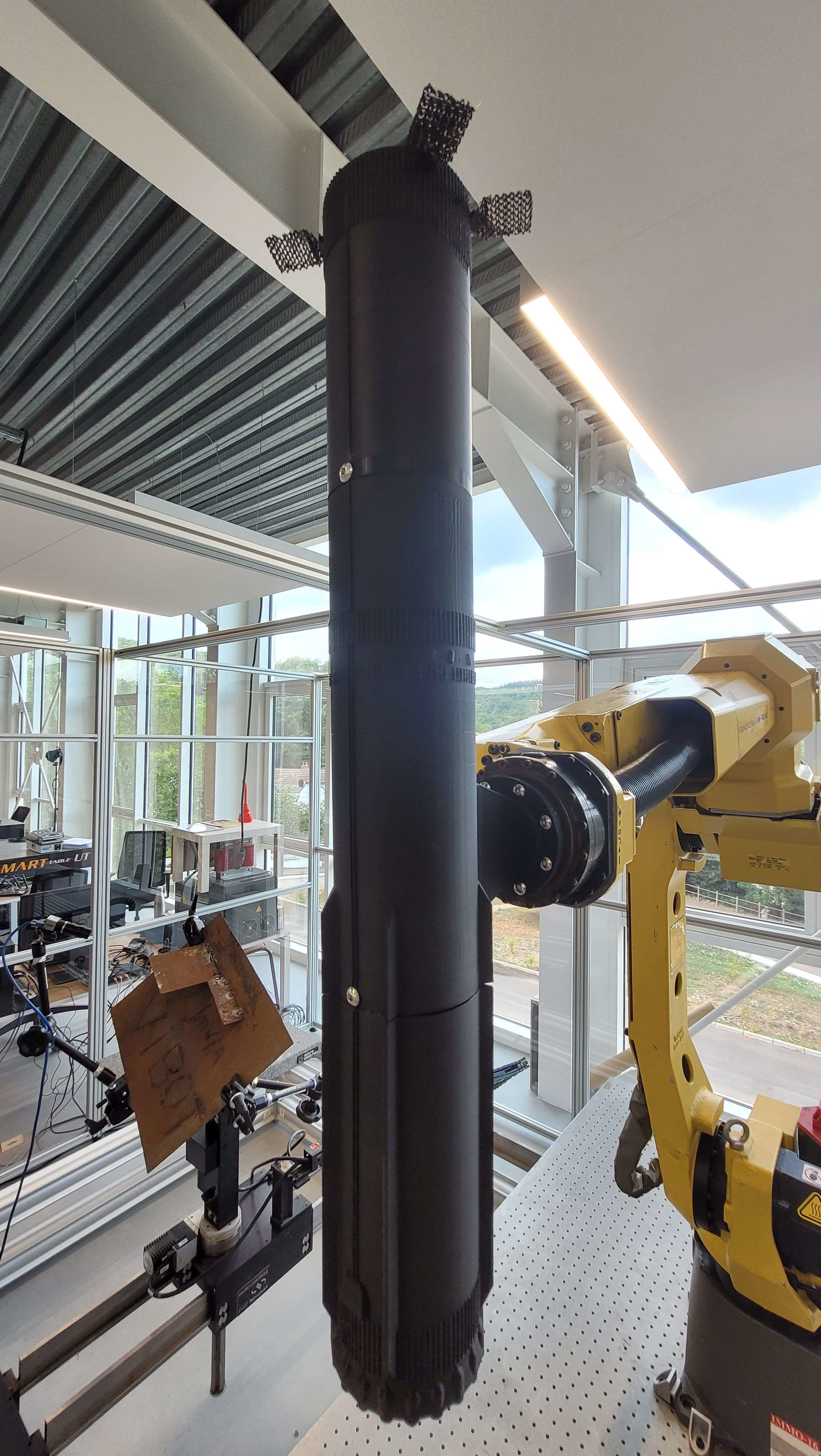
For this mockup, I need both aesthetic appeal (to be interesting to people) and a solid workhorse. The Super Heavy mockup needs to have 3 actuated grid fins, a way to measure its position relative to the tower mockup, wireless communications, onboard compute, and a mount to the FANUC arm. I made multiple booster mockups; here is the current one. Instead of a pure software simulation, the booster mock-up is physically mounted to the end of a FANUC industrial robotic arm. The arm executes the exact trajectory that the simulated catch maneuver would require, providing realistic inertial loads and kinematics.
Sensor data from the physical setup (encoders, force/torque if available) is fed back into the simulation loop. This closes the loop between the virtual vehicle dynamics and real mechanical hardware, exposing issues that pure simulation would miss.
Currently, the data still lacks processing (IMU drift), and the feedback loop is not done, I still do not know if I can make the communication fast enough for the simulation 50Hz control frequency.
Hardware-in-the-Loop Architecture
For this mockup, I need both aesthetic appeal (to be interesting to people) and a solid workhorse. The Super Heavy mockup needs to have 3 actuated grid fins, a way to measure its position relative to the tower mockup, wireless communications, onboard compute, and a mount to the FANUC arm. I made multiple booster mockups; here is the current one. Instead of a pure software simulation, the booster mock-up is physically mounted to the end of a FANUC industrial robotic arm. The arm executes the exact trajectory that the simulated catch maneuver would require, providing realistic inertial loads and kinematics.
Sensor data from the physical setup (encoders, force/torque if available) is fed back into the simulation loop. This closes the loop between the virtual vehicle dynamics and real mechanical hardware, exposing issues that pure simulation would miss.
Currently, the data still lacks processing (IMU drift), and the feedback loop is not done, I still do not know if I can make the communication fast enough for the simulation 50Hz control frequency.
FANUC Integration
FANUC is a global leader in industrial robotic manipulators, and we have two FANUC arms at Polytech: a small one for educational purposes, and a large one that had no real usage yet. I planned to participate in FANUC's national Olympiads, so I needed experience with their systems anyway. I am working with an R-30iA Mate controller, with an M-10iA/12S arm (V7.70 software). However, I need to make it work so I can stream real-time positions of the Super Heavy booster from ProxSim, following the exact same trajectory, without delay or jerk, and this is not what industrial robots are for: they are made for pre-programmed trajectories and logic.
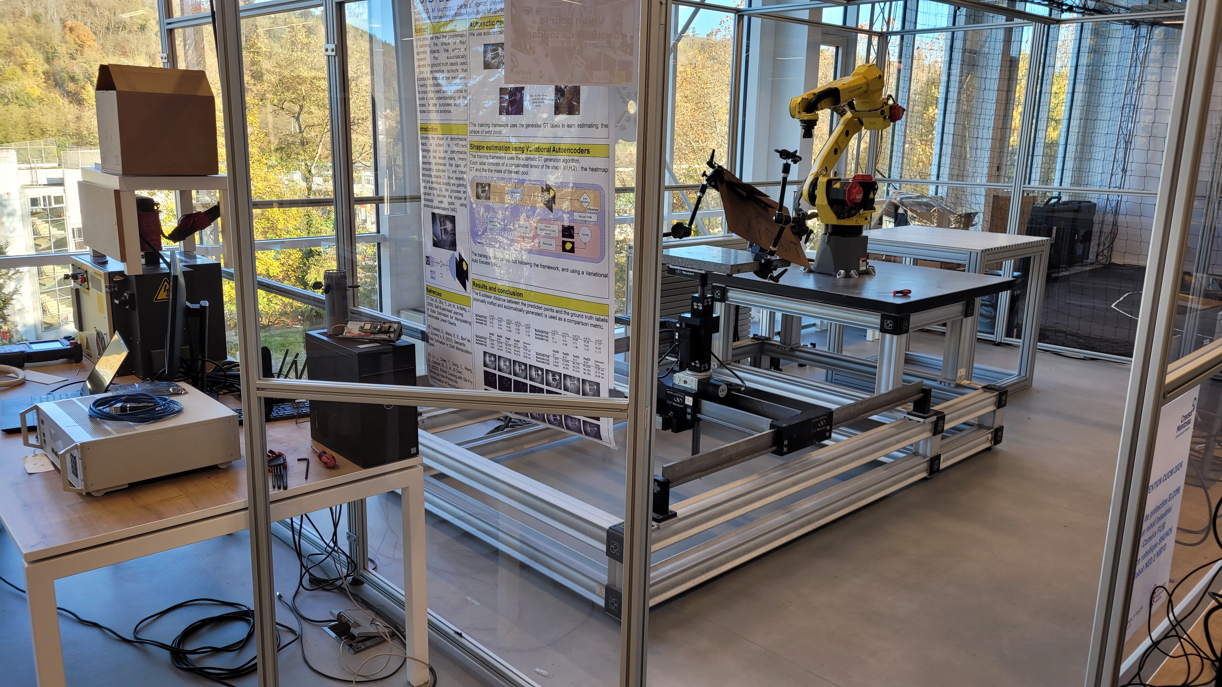
Wide view of the unused cell (mounted for a welding trajectory demo)
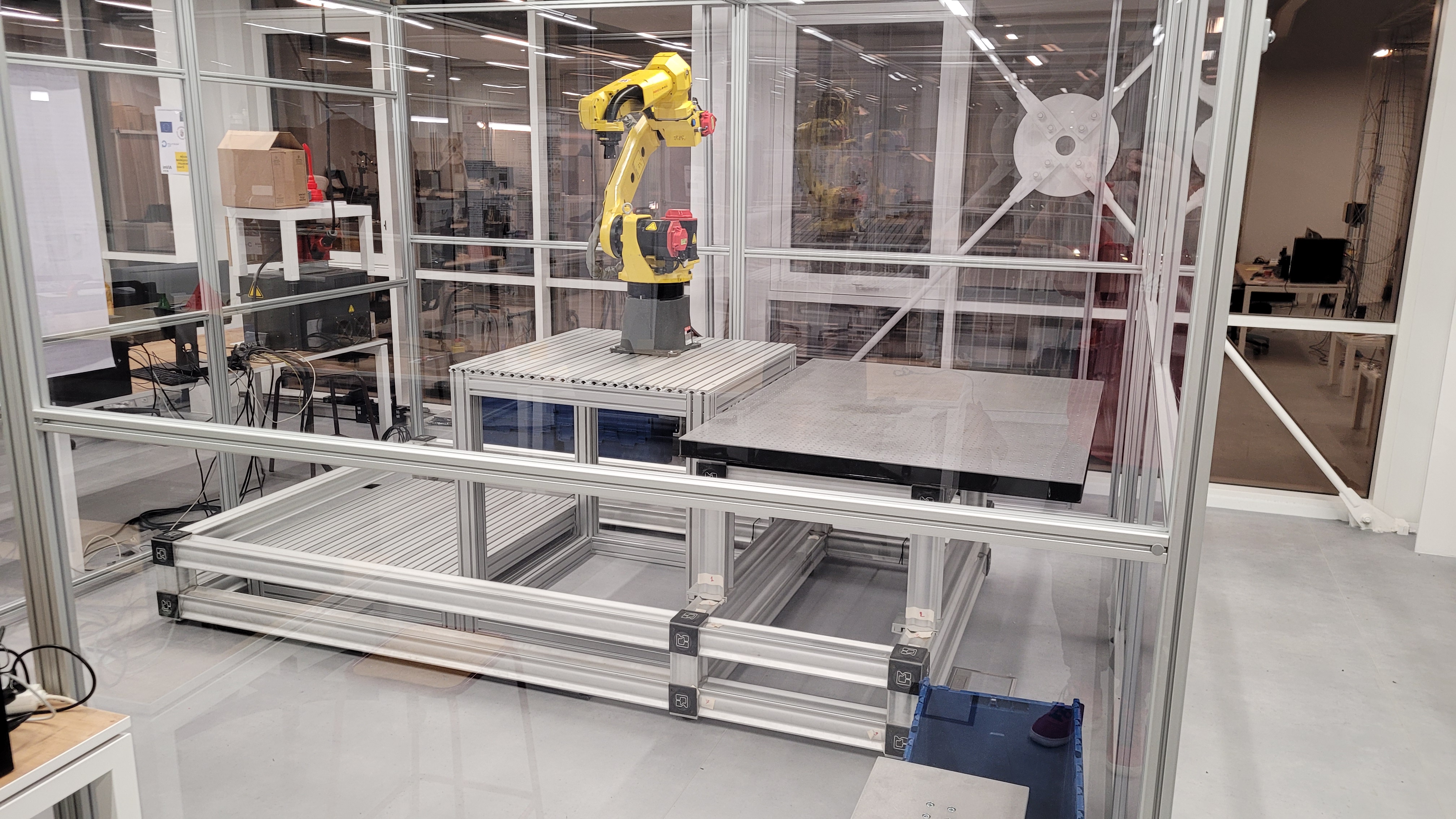
Wide view of the cell after a rework : a platform for usual robotics educational applications, and a lower strut to fix my Launch Tower mockup
I found a great library: fanucpy. It provides drivers (KAREL programs) to add to the robot, directions to set up an HTTP server on the controller, and a small Python program to run on a local computer. While it was a very good starting point, multiple features were missing: no continuous options, as all movements were executed individually (and not chained like in a regular FANUC program), commands could start multiple seconds after they were sent, and there was no management of user frames... So I reworked the whole library, from the low-level KAREL for the FANUC to the low-level C++ for the ProxSim library, to add a new spline functionality. The spline functionality is currently working on select test cases, but has yet to prove reliable once integrated into ProxSim; more testing is needed.
Here, I'm sending random positions at random intervals to the robot, and seeing how it handles them. Comparison between the first and the second (latest) version.
FANUC Spline V1 (Bézier curves). Stops are when no command arrives when the current one ends. Speed X2
FANUC Spline V2 (Hermite curves)
Technical details
How to have a continuous motion
The delay of multiple seconds is caused by the FANUC's own motion system. The brakes have to be released first, and then it can move. The brakes automatically activate a few seconds after the last motion concluded. The way fanucpy works by default is with a stack approach: each instruction (position, movement type, speed) has to be processed by the KAREL server and executed from a called TP program before the next can happen. I tried to use SKIP commands, but SKIPs always stop the robot before proceeding. My solution: have a TP program running continuously, waiting for instructions sent from the KAREL program. To manage interrupts (when the server receives a new command while the last one is not completed), I use two memory spaces, so KAREL can work on one while the TP program is looping on the other. Once KAREL has finished processing it, I make the TP program switch memory space.
About curves
If I sent every points at each simulation step, the FANUC may not handle it as it was not made for high-bandwidth communications, so an interpolation is necessary by the FANUC controller. Super Heavy being really heavy, it has a large inertia, which comes down to less jitter and an easier interpolation with less control points.
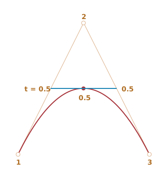
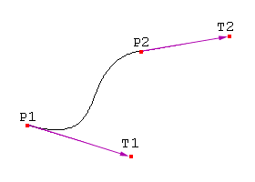
My first try was using Bézier curves, they are everywhere, they are simple, and I just had to find the control point that would make the start smooth with the current robot motion. However, Spline V1 was not smooth enough as scales were hard to get right. Bézier curves were never meant for movement. I then found Hermite curves. Hermite curves do not take a control point that corresponds directly to nothing except intersections of 2 lines in a 3D space, they take the start and end velocities instead. If it is late, the interpolation will push the robot faster to catch up. I then calculate, in the robot, the interpolation intermediate positions/speeds, write them to PRs, and send the signal to switch memories.
Bezier curves : intermediate physically meaningless points (but easy to compute, draw : foundations of computer graphics)
Hermite curves : only physically representative variables
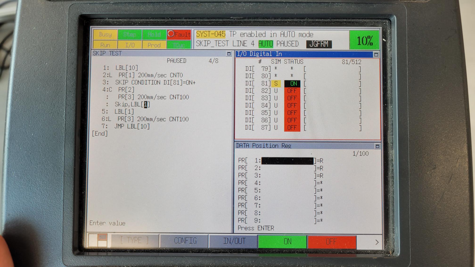
TP programs are interpreted, which means I can edit PRs at run time. However, FANUC's motion system reads ahead in the program to plan the trajectory. The "ahead" number of positions depends on the movement options: an "ACC" option makes the "ahead" count increase by one, and so does "CNT" when non-zero. So I keep track of the current movement index in memory, and start the next motion as if ahead by ~2 positions. This is the secret sauce to make the trajectory butter-smooth and avoid small hiccups/slowdowns.
FANUC Integration
FANUC is a global leader in industrial robotic manipulators, and we have two FANUC arms at Polytech: a small one for educational purposes, and a large one that had no real usage yet. I planned to participate in FANUC's national Olympiads, so I needed experience with their systems anyway. I am working with an R-30iA Mate controller, with an M-10iA/12S arm (V7.70 software). However, I need to make it work so I can stream real-time positions of the Super Heavy booster from ProxSim, following the exact same trajectory, without delay or jerk, and this is not what industrial robots are for: they are made for pre-programmed trajectories and logic.
Wide view of the unused cell (mounted for a welding trajectory demo)
Wide view of the cell after a rework : a platform for usual robotics educational applications, and a lower strut to fix my Launch Tower mockup
I found a great library: fanucpy. It provides drivers (KAREL programs) to add to the robot, directions to set up an HTTP server on the controller, and a small Python program to run on a local computer. While it was a very good starting point, multiple features were missing: no continuous options, as all movements were executed individually (and not chained like in a regular FANUC program), commands could start multiple seconds after they were sent, and there was no management of user frames... So I reworked the whole library, from the low-level KAREL for the FANUC to the low-level C++ for the ProxSim library, to add a new spline functionality. The spline functionality is currently working on select test cases, but has yet to prove reliable once integrated into ProxSim; more testing is needed.
Here, I'm sending random positions at random intervals to the robot, and seeing how it handles them. Comparison between the first and the second (latest) version.
FANUC Spline V1 (Bézier curves). Stops are when no command arrives when the current one ends. Speed X2
FANUC Spline V2 (Hermite curves)
Technical details
How to have a continuous motion
The delay of multiple seconds is caused by the FANUC's own motion system. The brakes have to be released first, and then it can move. The brakes automatically activate a few seconds after the last motion concluded. The way fanucpy works by default is with a stack approach: each instruction (position, movement type, speed) has to be processed by the KAREL server and executed from a called TP program before the next can happen. I tried to use SKIP commands, but SKIPs always stop the robot before proceeding. My solution: have a TP program running continuously, waiting for instructions sent from the KAREL program. To manage interrupts (when the server receives a new command while the last one is not completed), I use two memory spaces, so KAREL can work on one while the TP program is looping on the other. Once KAREL has finished processing it, I make the TP program switch memory space.
About curves
If I sent every points at each simulation step, the FANUC may not handle it as it was not made for high-bandwidth communications, so an interpolation is necessary by the FANUC controller. Super Heavy being really heavy, it has a large inertia, which comes down to less jitter and an easier interpolation with less control points.
My first try was using Bézier curves, they are everywhere, they are simple, and I just had to find the control point that would make the start smooth with the current robot motion. However, Spline V1 was not smooth enough as scales were hard to get right. Bézier curves were never meant for movement. I then found Hermite curves. Hermite curves do not take a control point that corresponds directly to nothing except intersections of 2 lines in a 3D space, they take the start and end velocities instead. If it is late, the interpolation will push the robot faster to catch up. I then calculate, in the robot, the interpolation intermediate positions/speeds, write them to PRs, and send the signal to switch memories.
Bezier curves : intermediate physically meaningless points (but easy to compute, draw : foundations of computer graphics)
Hermite curves : only physically representative variables
TP programs are interpreted, which means I can edit PRs at run time. However, FANUC's motion system reads ahead in the program to plan the trajectory. The "ahead" number of positions depends on the movement options: an "ACC" option makes the "ahead" count increase by one, and so does "CNT" when non-zero. So I keep track of the current movement index in memory, and start the next motion as if ahead by ~2 positions. This is the secret sauce to make the trajectory butter-smooth and avoid small hiccups/slowdowns.
Physical mockups
The goal of this project is to reverse-engineer a complex system, but also to prove to people that the tech exists for revolutionary transport. I need to interest people in my project, for visitors of science fairs, school visits, and so on. This means I have to make a mockup that is practical, easy to 3D-print (this is my only available manufacturing solution), and appealing.
As my project evolved, so did the Super Heavy booster's real design. Accounting for the usual iterations, I made 4 different versions.
Mockup 3 : Super Heavy V2
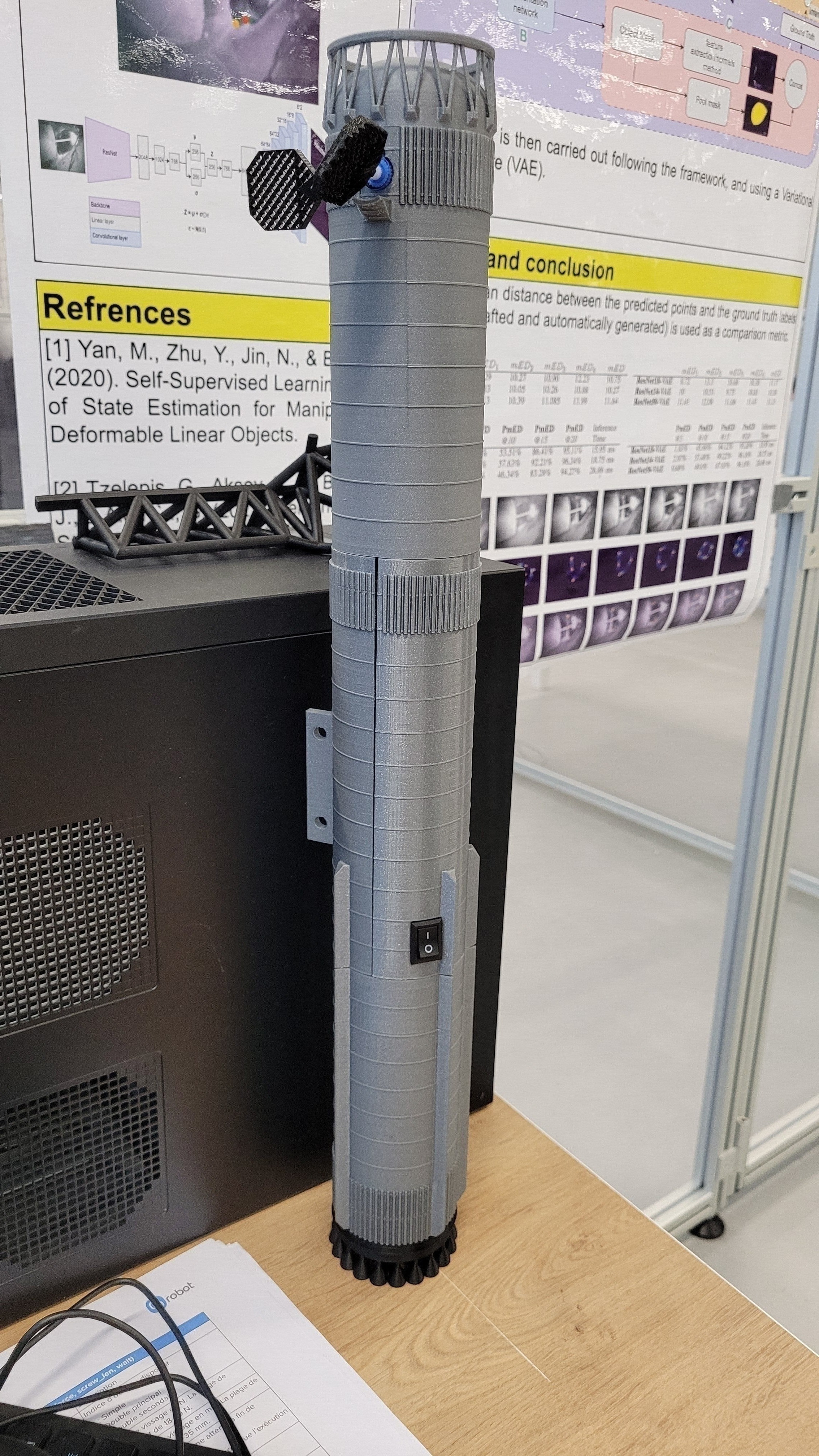
Mockup 4 : Super Heavy V3 : featuring rotating grid fins, twist-and-lock and good coloring.
It stands ~70 cm high, made in three sections (actuators, logic/comms, and battery). The three parts assemble using a twist-and-lock mechanism after the screws were too ugly and unreliable with heavy parts swinging around for hours.
Technical details
Features an ESP32 (used both for communications and IMU processing with low-pass filters; Kalman filters might come later). Made to fit and hold a whole breadboard, a large battery for autonomy, and a tight servo holder.
Printed on a BambuLab A1 printer, using 0.2 and 0.4 nozzles, with PLA (poor choice of material as it melted in the Sun...).
Physical mockups
The goal of this project is to reverse-engineer a complex system, but also to prove to people that the tech exists for revolutionary transport. I need to interest people in my project, for visitors of science fairs, school visits, and so on. This means I have to make a mockup that is practical, easy to 3D-print (this is my only available manufacturing solution), and appealing.
As my project evolved, so did the Super Heavy booster's real design. Accounting for the usual iterations, I made 4 different versions.
Mockup 3 : Super Heavy V2
Mockup 4 : Super Heavy V3 : featuring rotating grid fins, twist-and-lock and good coloring.
It stands ~70 cm high, made in three sections (actuators, logic/comms, and battery). The three parts assemble using a twist-and-lock mechanism after the screws were too ugly and unreliable with heavy parts swinging around for hours.
Technical details
Features an ESP32 (used both for communications and IMU processing with low-pass filters; Kalman filters might come later). Made to fit and hold a whole breadboard, a large battery for autonomy, and a tight servo holder.
Printed on a BambuLab A1 printer, using 0.2 and 0.4 nozzles, with PLA (poor choice of material as it melted in the Sun...).
Visual Documentation
Early visuals from the simulation environment, cell programming, and hardware setup. These assets will be replaced or expanded with higher-quality captures, diagrams, and annotated footage in later iterations.
Overall view of the test cell and catch envelope
Program experimenting with path interruption and look-aheads.
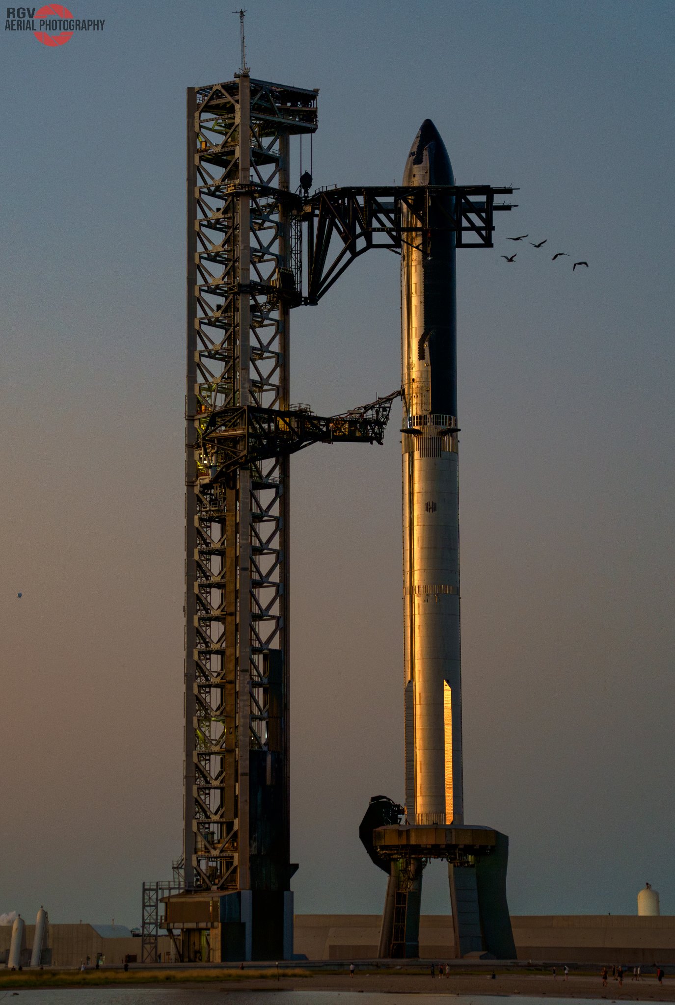
Reference full-stack vehicle
IFT-5 recap footage used for maneuver reference and timingVisual Documentation
Early visuals from the simulation environment, cell programming, and hardware setup. These assets will be replaced or expanded with higher-quality captures, diagrams, and annotated footage in later iterations.
Overall view of the test cell and catch envelope
Program experimenting with path interruption and look-aheads.
Reference full-stack vehicle
IFT-5 recap footage used for maneuver reference and timing
Control Approach
During unpowered descent, Super Heavy guides itself with its three grid fins, and its own large body inducing a lift. Aerodynamics studies are to be concluded, to estimate the drag of the booster and the torque created by the gridfins. I began to learn OpenFOAM, but as this work is far from my Robotics domain, I let AI do most of the implementation of aerodynamics in ProxSim and will let it find the constants in simulations, it has yet to be done.
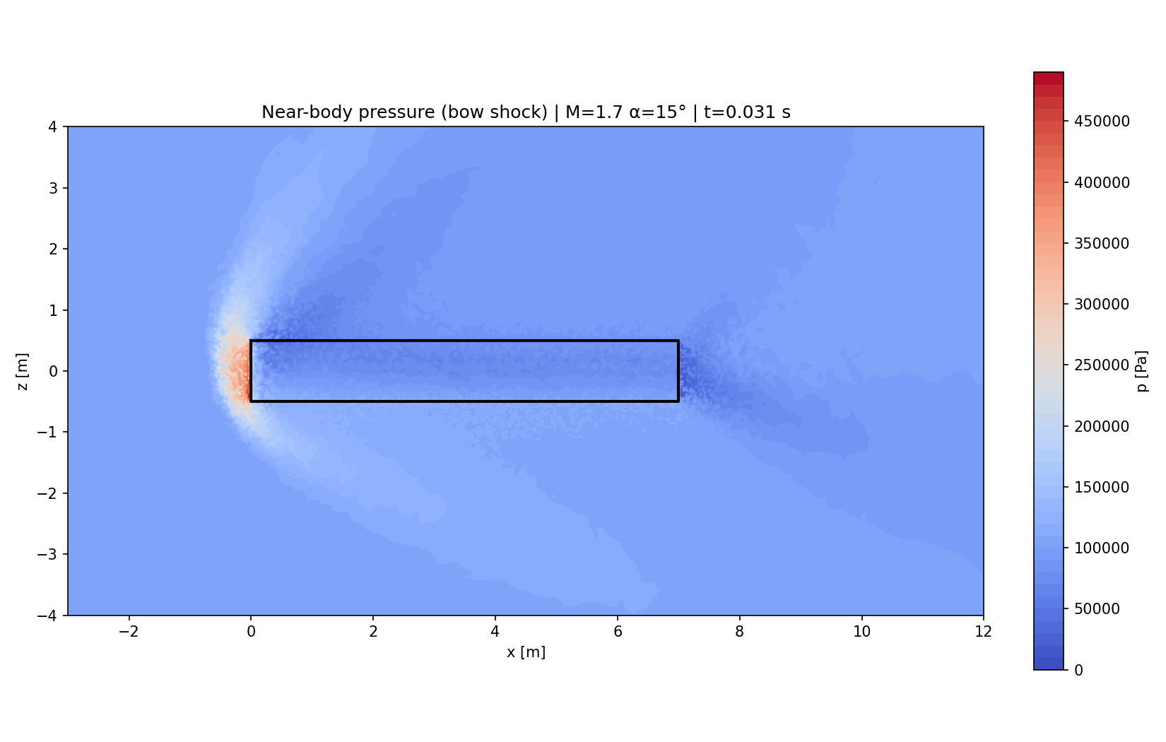
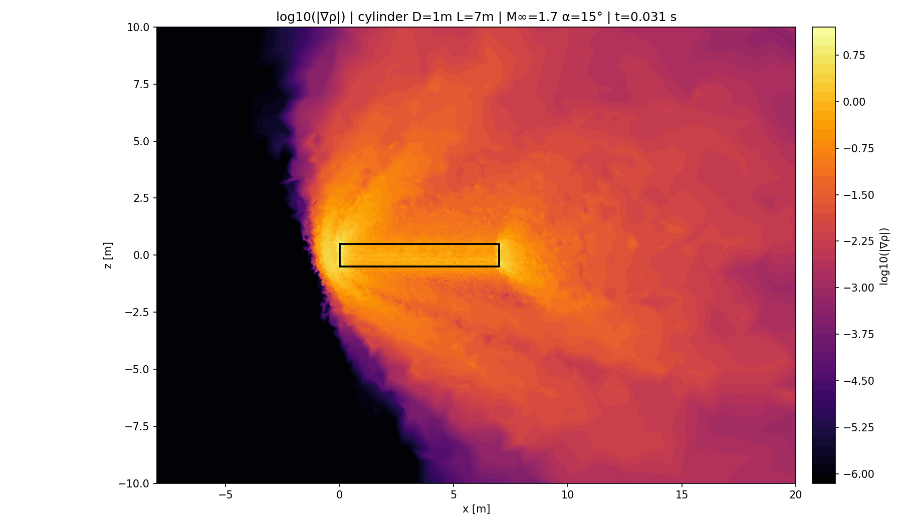
Simple CFD simulation done by a Grok Bot using OpenFOAM
Simple CFD simulation done by a Grok Bot using OpenFOAM
Control Approach
During unpowered descent, Super Heavy guides itself with its three grid fins, and its own large body inducing a lift. Aerodynamics studies are to be concluded, to estimate the drag of the booster and the torque created by the gridfins. I began to learn OpenFOAM, but as this work is far from my Robotics domain, I let AI do most of the implementation of aerodynamics in ProxSim and will let it find the constants in simulations, it has yet to be done.
Simple CFD simulation done by a Grok Bot using OpenFOAM
Simple CFD simulation done by a Grok Bot using OpenFOAM